Simple Overview Statistical Comparison Tests
The vast majority of statistical tests really just
- compare several populations on one variable or
- compare several variables in one population.
Now, if we add to this comparison
- the number of variables or populations and
- the measurement levels of our variables
then choosing the appropriate statistical test suddenly becomes remarkably easy.
The overviews below also nicely visualize how basic tests relate to each other. Click the links in the tables for a simple visualization and some key points for each test.
The overviews below also nicely visualize how basic tests relate to each other. Click the links in the tables for a simple visualization and some key points for each test.
A. Comparing Groups of Cases
B. Comparing Variables
| OUTCOME VARIABLE(S) | 1 VARIABLE | 2 VARIABLES | 3(+) VARIABLES |
|---|---|---|---|
| Dichotomous | Z-Test for One Proportion or Binomial Test | McNemar Test | Cochran Q test |
| Nominal | Chi-Square Goodness-of-Fit Test | (None) | (None) |
| Ordinal | Sign Test for One Median | Wilcoxon Signed-Ranks Test or Sign Test for 2 Related Medians | Friedman Test |
| Metric (“scale”) | One Sample T-Test | Paired Samples T-Test | Repeated Measures ANOVA |
Z Test for One Proportion
Null Hypothesis
The population proportion for some value is equal to some hypothesized proportion, p0.
Assumptions
- Independent and identically distributed variables.
- p0*n and (1 - p0)*n must both be > 5, where p0 denotes the hypothesized population proportion and n the sample size.6 See notes.
Where in SPSS?
Not available. However, see below.
Notes
- The z-test yields an approximate (“asymptotic”) p-value that's more accurate insofar as the sample size is larger and p0 is closer to 0.5. Different authors suggest different rules for when the approximation is accurate enough.4
- The binomial test has the same null hypothesis but can't come up with a confidence interval for a proportion or a 2-tailed p-value unless p0 = 0.5. On the other hand, the binomial test always yields an exact p-value and does not require any minimum sample size.
Further Reading
Binomial Test
Null Hypothesis
The population proportion for some value is equal to some hypothesized proportion, p0.
Assumptions
- Independent and identically distributed variables.
Where in SPSS?
Notes
The binomial test has the same null hypothesis but can't come up with a confidence interval for a proportion or a 2-tailed p-value unless p0 = 0.5. On the other hand, the binomial test always yields an exact p-value and does not require any minimum sample size.
Further Reading
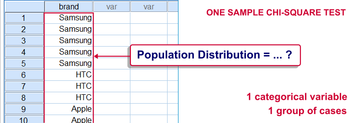
Chi-Square Goodness-of-Fit Test
Null Hypothesis
The population distribution of a categorical variable is identical to some hypothesized distribution.
Assumptions
- Independent and identically distributed variables.
- Less than 20% of the expected frequencies are < 5.4
- None of the expected frequencies is < 1.
Where in SPSS?
Notes
- For dichotomous variables, a z-test for one proportion or a binomial test is preferable.
- This test is known as the one-sample chi-square test in SPSS.
Further Reading
Sign Test for One Median
Null Hypothesis
The population median of some variable is equal to a hypothesized value, η0.
Assumptions
- Independent and identically distributed variables.
Where in SPSS?
Not available. However, you can RECODE the test variable into signs (plus and minus) that indicate if each data value is larger or smaller than η0 and use a binomial test with p0 = 0.5.
Alternatively, add η0 as a new variable (or actually a constant) to your data and use a sign test for 2 related medians.
Alternatively, add η0 as a new variable (or actually a constant) to your data and use a sign test for 2 related medians.
Further Reading
One Sample T-Test
Null Hypothesis
The population mean of some variable is equal to a hypothesized value, μ0.
Assumptions
- Independent and identically distributed variables.
- The test variable is normally distributed in the population. For reasonable sample sizes (say, n > 25), this assumption is not needed.3
Where in SPSS?
The easiest option is 
 .
.

 .
.Further Reading
Z-Test for 2 Independent Proportions
Null Hypothesis
The difference between two independent proportions, p1 and p2 is equal to some hypothesized value, δ0. “Independent proportions” refers to proportions of one variable in two (disjoint) populations. Since δ0 is often zero, we'll simplify this to both proportions being equal.
Assumptions
- Independent and identically distributed variables.
- p1*n1, (1-p1)*n1, p2*n2 and (1-p2)*n2 are all > 5, where p and n denote the two test proportions and their related sample sizes.6
Where in SPSS?
Not available. However, see below.
Further Reading
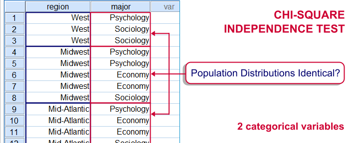
Chi-Square Independence Test
Null Hypothesis
Two categorical variables are statistically independent in some population. Or, equivalently, the population distributions of some categorical variable are identical for a number of subpopulations defined by a second categorical variable.
Assumptions
- Independent and identically distributed variables.
- All expected cell frequencies ≥ 5.1
Where in SPSS?


Alternatively, for 2 variables named var1 and var2, just typecrosstabs var1 by var2/statistics chisq.into your syntax editor window and run it.
Notes
- For two dichotomous variables, use a z-test for 2 independent proportions instead. It yields an identical significance level but adds to that a confidence interval for the difference between the proportions.
- This test can be extended to 3 or more variables. In this case we speak of loglinear analysis. The chi-square independence test is technically a special (simplest possible) case of a loglinear model.
Further Reading
Mann-Whitney Test
Null Hypothesis
The mean ranks on some variable are equal for two populations. Some textbooks propose that “the population distribution of some variable is identical in 2 populations except for the central tendency”3. We don't like this formulation because “central tendency” is vague (it certainly isn't a mean or a median) and therefore unmeasurable.
Assumptions
Independent and identically distributed variables.
Where in SPSS?
Notes
- This test is also known as the Wilcoxon (rank-sum) test, which is not to be confused with the Wilcoxon signed-ranks test.
- The Mann-Whitney test is typically used instead of the independent samples t-test when the latter’s assumptions aren't met.
- On skewed variables, the MW test may sometimes be more powerful than the independent samples t-test.
Further Reading
Median Test for 2(+) Independent Medians
Null Hypothesis
Two or more (disjoint) populations all have identical medians on some variable.
Assumptions
Independent and identically distributed variables (sometimes referred to as “independent observations”).
Where in SPSS?
On recent SPSS versions, we prefer using 


Notes
- The median test is not a very powerful test. This is because it only evaluates if data values are either larger or smaller than the median. It thus ignores the magnitudes of such differences.
- An alternative that does take these into account is the Mann-Whitney test for two independent samples.
- For K (meaning 3 or more) independent samples, consider the Kruskal-Wallis test instead of the median test.
Further Reading
Independent Samples T-Test
Null Hypothesis
Some variable has identical means in two (disjoint) populations.
Assumptions
- Independent observations or, more precisely, Independent and identically distributed variables.
- Normality: the test variable must be normally distributed in both populations. This assumption is mostly important for smaller sample sizes, say n < 25 for either sample.6
- Homogeneity: the variance of the test variable must be equal in both populations being compared. Violation of this assumption is more serious insofar as the 2 sample sizes are different.
Where in SPSS?
The easiest option is 


Notes
- If the normality assumption is seriously violated and sample sizes are small, consider using the Mann-Whitney test intstead of the t-test.6
- By default, SPSS includes Levene's test in the output which tests the assumption of equal variances (not the main null hypothesis of equal population means). Generally, p < 0.05 for the Levene test is seen as evidence that the assumptions of equal variances does not hold.
- The assumption of equal variances not holding (but the normality assumption being met) is known as the Behrens-Fisher problem. One way of dealing with it is an adjustment of df (degrees of freedom) known as the Welch-Satterthwaithe solution.3 The result is found in SPSS’ output under “equal variances not assumed” (shown below).
 P < 0.05 for Levene’s test so the assumption of equal variances is not met.
 We therefore report the second row of the t-test results denoted by “equal variances not assumed”.
 Note how df has been adjusted according to the Welch correction.
 We'll report something like “a t-test did not show the means to be statistically significantly different, t(29) = 1.55, p = 0.133”.
Further Reading
Null Hypothesis
The population proportion for some value is equal to some hypothesized proportion, p0.
Assumptions
- Independent and identically distributed variables.
- p0*n and (1 - p0)*n must both be > 5, where p0 denotes the hypothesized population proportion and n the sample size.6 See notes.
Where in SPSS?
Not available. However, see below.
Notes
- The z-test yields an approximate (“asymptotic”) p-value that's more accurate insofar as the sample size is larger and p0 is closer to 0.5. Different authors suggest different rules for when the approximation is accurate enough.4
- The binomial test has the same null hypothesis but can't come up with a confidence interval for a proportion or a 2-tailed p-value unless p0 = 0.5. On the other hand, the binomial test always yields an exact p-value and does not require any minimum sample size.
Further Reading
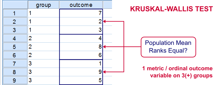
Kruskal-Wallis Test
Null Hypothesis
The mean ranks of some variable are all equal over 3 or more (disjoint) subpopulations.1
Other authors propose that the population distributions of some variable are identical over 3 or more (disjoint) subpopulations1 or even that the medians are identical over subpopulations.3 We feel the first formulation is preferable but opinions differ.
Other authors propose that the population distributions of some variable are identical over 3 or more (disjoint) subpopulations1 or even that the medians are identical over subpopulations.3 We feel the first formulation is preferable but opinions differ.
Assumptions
Independent and identically distributed variables (or, less precisely, independent observations).
Our preferred dialog is under 


Notes
- The KW test is mostly used instead of a one-way ANOVA when the latter’s assumptions (especially normality) aren't met by the data.
- The test statistic, Kruskal-Wallis H, is incorrectly denoted as Chi-Square in SPSS.
- The sampling distribution of Kruskal-Wallis H is complex but can be approximated by a chi-square distribution if samples sizes are sufficient. A rule of thumb is all ni ≥ 4, which will probably always be the case.6
Further Reading
One-Way ANOVA
Null Hypothesis
The population means for some variable are all equal over 3 or more (disjoint) subpopulations.
Assumptions
- Independent observations (precisely: independent and identically distributed variables).
- Homogeneity: the population variances are all equal over subpopulations. Violation of this assumption is less serious insofar as all sample sizes are equal.6
- Normality: the test variable must be normally distributed in each subpopulation. This assumption becomes less important insofar the sample sizes are larger.
Where in SPSS?
SPSS offers many way for running a one-way ANOVA. For a very basic test, try 

If you'd like some more detailed output, including partial eta squared (a measure for effect size), go for


If you'd like some more detailed output, including partial eta squared (a measure for effect size), go for


Notes
- One-way ANOVA only tests whether all population means are equal. If this doesn't hold, you may use a post-hoc test such as Tukey’s HSD to find out exactly which means are different.
- In practice, two or even more factors are often included in the model simultaneously. This extends one-way ANOVA to two way ANOVA or even multiway ANOVA.
Further Reading
- ANOVA - What Is It?
- SPSS One-Way ANOVA
- SPSS - One Way ANOVA with Post Hoc Tests Example
- SPSS Two Way ANOVA - Basics Tutorial
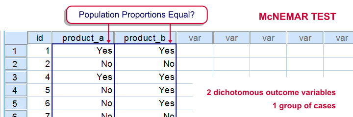
McNemar Test
Null Hypothesis
The population proportions with which some value occurs in two variables are equal.
Assumptions
Independent and identically distributed variables or, less precisely, independent observations.
Where in SPSS?
We prefer using the dialog under 


Further Reading
Wilcoxon Signed-Ranks Test
Null Hypothesis
Two variables are identically distributed in some population.3 Or, alternatively, the population median of difference scores is zero.1
Assumptions
Independent and identically distributed variables.
Where in SPSS?
We prefer using the dialog under 


Notes
- Don't confuse the Wilcoxon Signed-Ranks test with Wilcoxon’s Rank-Sum test, which is an alias for the Mann-Whitney test. For this reason, the term “Wilcoxon test” is better avoided.
- The test statistic, Wilcoxon W+, has a complex sampling distribution. For sample sizes > 15, it may be approximated by a normal distribution.6 The significance level resulting from this approximation is denoted as “Asymp. Sig. (2-tailed)” in SPSS.
Further Reading
Sign Test for 2 Related Medians
Null Hypothesis
The population medians for two variables are equal.
Assumptions
Independent and identically distributed variables.
Where in SPSS?
The simplest option is 


Notes
Like all tests on medians, this test suffers from low power. It only takes into account if difference scores are larger or smaller than zero but it ignores how much larger or smaller. Therefore, the Wilcoxon signed-ranks test is usually a better alternative for the sign test.
Further Reading
Paired Samples T-Test
Null Hypothesis
Two variables have equal population means.
Assumptions
- Independent observations (or precisely: independent and identically distributed variables).
- Difference scores between the two variables must be normally distributed in the population. This assumption is less important insofar as the sample size is larger and may perhaps be ignored altogether if n > 25 or 30.
Where in SPSS?
The standard approach is 

For sample sizes < 25 or so, perhaps COMPUTE difference scores manually and first run a histogram on them to check if the normality assumption has been satisfied. If you'd like to test many variables, speed things up with DO REPEAT. You can now test if each variable holding difference scores has a population mean of zero with


For sample sizes < 25 or so, perhaps COMPUTE difference scores manually and first run a histogram on them to check if the normality assumption has been satisfied. If you'd like to test many variables, speed things up with DO REPEAT. You can now test if each variable holding difference scores has a population mean of zero with


Notes
- The paired-samples t-test is equivalent to a one-sample t-test on difference scores.
- If the normality assumption is severely violated in small sample sizes (say, n < 25), consider using the Wilcoxon signed-ranks test instead of the t-test.
Further Reading
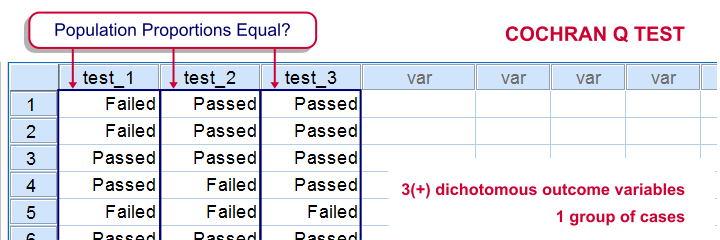
Cochran’s Q Test
Null Hypothesis
The population proportions with which some value occurs in 3 or more variables are all equal.7
Assumptions
Independent and identically distributed variables.
Where in SPSS?
Our preferred approach is 


Further Reading
Friedman Test
Null Hypothesis
Three or more variables have identical population distributions. However, the Friedman test mainly detects if the scores of all test variables are equally large. It won't detect other differences such as unequal standard deviations or skewnesses over variables.
Assumptions
Independent and identically distributed variables.
Where in SPSS?
Our preferred approach is 


Notes
- The Friedman test comes close to a repeated measures ANOVA on within-subjects rank numbers. It's mainly used instead of repeated measure ANOVA because it requires fewer assumptions on your data.
- The test statistic, Friedman’s Q, is incorrectly denoted as “Chi-Square” in SPSS’ output;
- The sampling distribution of Q is complex. It may be approximated by a chi-square distribution if the sample size is reasonable.
- By default, SPSS only reports this approximate significance level (“Asymp. Sig.”). For a small sample size, it may be wildly off. In this case, the exact p-value is needed but this requires the SPSS exact tests option. Alternatively, compute Friedman’s Q in SPSS and look up its exact p-value in a table.
Further Reading
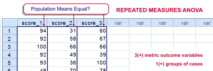
Repeated Measures ANOVA
Null Hypothesis
The population means of 3 or more variables are all equal.
Assumptions
- Independent and identically distributed variables (“independent observations”).
- Normality: the test variables follow a multivariate normal distribution in the population.
- Sphericity: the variances of all difference scores among the test variables must be equal in the population.2
Where in SPSS?


Repeated measures ANOVA is only available if you have SPSS’ advanced statistics module installed.
Notes
- If the normality assumption is severely violated in a small sample, consider using a Friedman test instead.
- By default, SPSS includes Mauchly’s test in the output which tests the sphericity assumption.
- If Mauchly’s test indicates a severe violation of sphericity, we'll report corrected ANOVA results denoted by Greenhouse-Geisser or Huynh-Feldt.
Further Reading
- Repeated Measures ANOVA - Simple Introduction
- SPSS Repeated Measures ANOVA
- SPSS Repeated Measures ANOVA - Example 2
References
- Agresti, A. & Franklin, C. (2014). Statistics. The Art & Science of Learning from Data. Essex: Pearson Education Limited.
- Field. Discovering Statistics with IBM SPSS Newbury Park, CA: Sage.
- Howell, D.C. Statistical Methods for Psychology (5th ed.). Pacific Grove CA: Duxbury.
- Siegel, S. & Castellan, N.J. (1989). Nonparametric Statistics for the Behavioral Sciences (2nd ed.). Singapore: McGraw-Hill.
- Van den Brink, W.P. & Koele, P. (1998). Statistiek, deel 2 [Statistics, part 2]. Amsterdam: Boom.
- Van den Brink, W.P. & Koele, P. (2002). Statistiek, deel 3 [Statistics, part 3]. Amsterdam: Boom.
- Wijnen, K., Janssens, W., De Pelsmacker, P. & Van Kenhove, P. (2002). Marktonderzoek met SPSS: statistische verwerking en interpretatie [Market Research with SPSS: statistical processing and interpretation]. Leuven: Garant Uitgevers.


